I have recently been exposed to more problems where an in depth understanding of signal processing and spectral analysis would be extremely valuable. These problems include constructing mobility endpoints from high frequency wrist worn accelerometer data, deriving RR-intervals from raw PPG waveform signals, and audio analysis work for speech related biomarker development.

This blog post explores the Karplus Strong Algorithm which is a method of constructing signals that sound like stringed instruments. It’s a nice example of some simple DSP techniques applied to sound data that generate realistic sounding signals. Hopefully you will find it interesting.

As I wrote this blog post I pulled ideas from the following sources: 1. The original Karplus-Strong paper: Digital Synthesis of Plucked-String and Drum Timbres 2. I also borrowed heavily from this excellent blog 3. And also this excellent blog 4. I also used some information from the Coursera DSP Course

A quick refresher on recursive signals

The Karplus Strong Algorithm has some recursive elements, so it’s worthwhile refreshing some of the details on recursive signals.

Suppose we have the following signal: \[y[n] = \alpha y[n-k] + \bar x[n]\]

Note that the signal is recursive, e.g. \(y[n]\) is a function of past lagged values of itself. Let’s choose a few concrete parameters and play with this signal sequence. Let: - \(\alpha = 0.7\) - \(\bar x[n] = \delta [n]\) where \(\delta [n]\) is the unit impulse function, also known as the Dirac-delta function

Let’s code this up in order to analyze this signal.

import numpy as np
import matplotlib.pyplot as plt
import seaborn as sns

%matplotlib inline

index = np.arange(-100, 100)
delta = np.zeros(len(index))
delta[index==0] = 1

plt.stem(index, delta, use_line_collection=True)
plt.tight_layout()
sns.despine()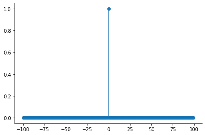

# We'll define y[n] to be zero for n < 0 
def y(n, k, alpha, x):
    """Generate a recursive signal y from a fixed length signal x, a lag k, and a decay factor alpha."""
    i = 0
    yn = np.array(x[n==0])
    for i in range(n[-1]):
        if i - k < 0:
            y_lag = 0
        else:
            y_lag = yn[i-k]
        yi = np.array([alpha*y_lag + x[i]])
        yn = np.concatenate([yn, yi])
    return yn

fig = plt.figure(figsize=(16, 4))

for i, alpha in enumerate([1, 0.8, 0.9, 1.2]):
    ax = fig.add_subplot(2, 2, i+1)
    yn = y(index, 3, alpha, delta)
    ax.stem(index[index>=0], yn, use_line_collection=True)
    ax.title.set_text('$ \\alpha$ = {}'.format(alpha))

plt.tight_layout()
sns.despine()

We can see that the recursive sequence results in a period signal, where the \(\alpha\) parameter controls the decay of the signal towards zero. That’s a curious phenomenon, given that the only nonzero portion of the input signal \(\bar x[n]\) is at \(n=0\).

Building a basic music synthesizer

Let’s move on to building a few sounds using the mathematical model we outlined above. One way of creating a music synthesizer is a concept known as wave table synthesis. The general idea is that we can produce a wave table, which is a periodic wave form in its sample representation (e.g. an array of values corresponding the one period of the signal), and we can loop through this waveform at different speeds to get different wave forms. Let’s build a basic synthesizer function.

from IPython.display import display, Audio

def synthesize(sampling_rate, wave_table, n_samples):
    """Construct a new waveform using a repeating periodic wave table.
    Source: https://flothesof.github.io/Karplus-Strong-algorithm-Python.html, with some modifications.
    """
    sample = np.zeros(n_samples)
    si = 0
    for i in range(n_samples):
        si += sampling_rate
        si = si % wave_table.size
        sample[i] = wave_table[si]
        si += 1
    return sample

# Sampling rate
fs = 8000

t = np.linspace(0, 1, num=fs)
wavetable = np.sin(np.sin(2 * np.pi * t))

plt.plot(wavetable)
plt.title('Wavetable')
plt.xlabel('Sample number')
plt.tight_layout()
sns.despine()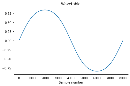

fig = plt.figure(figsize=(16, 6))

sampling_speeds = [110, 220, 440, 880]

for i, f in enumerate(sampling_speeds):
    sample = synthesize(f, wavetable, 2*fs)
    ax = fig.add_subplot(2, 2, i+1)
    ax.plot(sample[:500])
    ax.title.set_text('Synthesized Signal: Sampling Rate: {}'.format(f))
    display(Audio(sample, rate=fs))
    
plt.tight_layout()
sns.despine()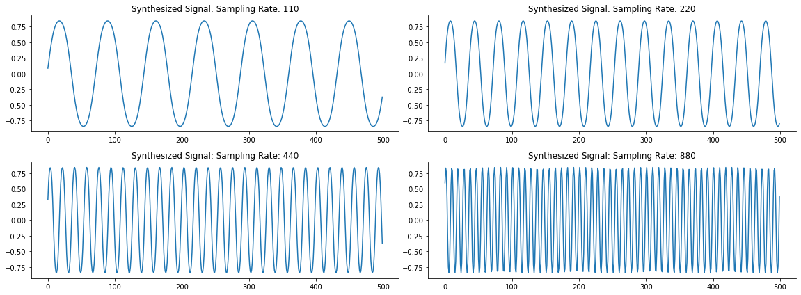

You can see that as we double the sampling speed/rate, the period of the synthesized waveform is cut in half. Also, listening to the sounds you can tell that the pitch increases by an octave. While this is a nice exercise, it isn’t a nice sound. We can explore other wave tables as well including the triangular wave, square wave, and the sawtooth wave.

import scipy.signal as signal

N = 110
t = np.linspace(0, 1, N)
sawtooth_wt = signal.sawtooth(2 * np.pi * t)
triangular_wt = signal.triang(N)
square_wt = signal.square(2 * np.pi * t)

sample = synthesize(f, sawtooth_wt, 2*fs)
plt.plot(sawtooth_wt[:N])
plt.title('Sawtooth wavetable')
plt.xlabel('Sample Number')

Audio(sample, rate=fs)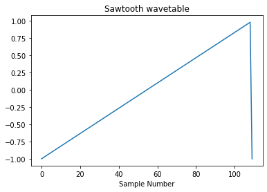

sample = synthesize(f, triangular_wt, 2*fs)
plt.plot(triangular_wt[:N])
plt.title('Triangular wavetable')
plt.xlabel('Sample Number')

Audio(sample, rate=fs)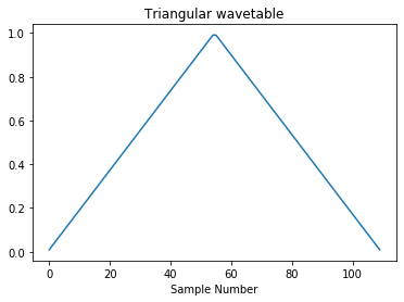

sample = synthesize(f, square_wt, 2*fs)
plt.plot(square_wt[:N])
plt.title('Square wavetable')
plt.xlabel('Sample Number')

Audio(sample, rate=fs)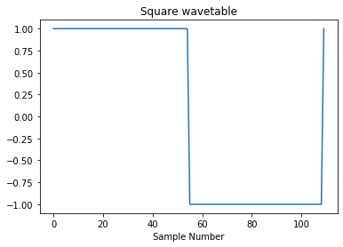

The waveforms are interesting and distinctly different, but sound terrible. Natural sounds vary over time, and aren’t purely periodic. Enter the Karplus Strong algorithm.

The Karplus Strong Algorithm

The original Karplus Strong “plucked string” algorithm has the following implementation:

\[Y_{t} = \frac{1}{2}[Y_{t-p} + Y_{t-p-1}]\]

Essentially it’s a simple recursion formula where successive values of \(Y\) are averaged together. This averaging results in a decay of the signal.

def karplus_strong(wavetable, n_samples):
    """
    Synthesizes a new waveform from an existing wavetable, modifies last sample by averaging.
    Source: https://flothesof.github.io/Karplus-Strong-algorithm-Python.html, with some modifications.
    """
    samples = []
    current_sample = 0
    previous_value = 0
    wavetable = wavetable.copy()
    while len(samples) < n_samples:
        wavetable[current_sample] = 0.5 * (wavetable[current_sample] + previous_value)
        samples.append(wavetable[current_sample])
        previous_value = samples[-1]
        current_sample += 1
        current_sample = current_sample % wavetable.size
    return np.array(samples)

# Demonstrate the decay using the square wave form
sample = karplus_strong(square_wt, 2*fs)
plt.plot(sample)
plt.xlabel('Sample Number');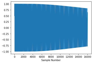

for wt in [square_wt, sawtooth_wt, triangular_wt]:
    sample = karplus_strong(wt, 2*fs)
    display(Audio(sample, rate=fs))

This is a significantly more interesting sound already! The original paper suggest using a wave table of random values drawn from the set {-1, 1} to initialize the algorithm.

wavetable_size = fs // 55

wavetable = np.random.choice([-1, 1], wavetable_size).astype(np.float32)

plt.plot(wavetable)
plt.tight_layout()
sns.despine()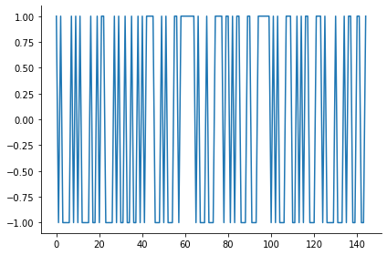

sample = karplus_strong(wavetable, 2 * fs)

Audio(sample, rate=fs)

Sounds like a guitar string being plucked! Very cool. The paper describes various extensions to the algorithm, including a modification that makes drum like noises. Additionally, these constructed signals can be overlayed to make realistic sounding guitar riffs.