Model performance under volatile outcome prevalence

Many of the machine learning problems I have worked on are disease detection or symptom detection problems. For example: predict whether an individual has flu given signals in their wearable data. What makes these problems particularly tricky (especially in infectious disease) is that often the underlying prevalence of disease rapidly changes. This rapid change means that you very quickly get a mismatch between your training and testing data. It also means that you need to be very judicious about which model evaluation metrics you choose to track, because many metrics will be insensitive to this form of distribution drift.

When analyzing this phenomenon, a helpful starting place is to look at Bayes’ Theorem:

\[P(+ | Test^{+}) = \frac{P(Test^{+} | +) P(+)}{P(Test^{+})}\]

In the above formulation the posterior probability is the precision of the model, and the term \(P(+)\) (known as the prior in Bayesian parlance) is the prevalence of the disease. From this basic analysis we would expect the precision of any model to increase proportionally to the underlying prevalence of the positive class.

We can simulate this phenomenon and verify it holds empirically.

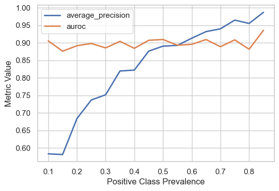
import numpy as np
import pandas as pd
import seaborn as sns
import matplotlib.pyplot as plt

from sklearn.datasets import make_classification
from sklearn.linear_model import LogisticRegression
from sklearn.ensemble import RandomForestClassifier
from sklearn.metrics import (
    precision_score, 
    average_precision_score,
    recall_score,
    roc_auc_score,
    classification_report)
from sklearn.model_selection import train_test_split

sns.set(style='whitegrid')
np.random.seed(42)

def resample_with_prevalence(X, y, sample_size, prevalence):
    """ Resamples the dataset X, y to have the desired prevalence of the positive class.
    
    Parameters:
    X (numpy.ndarray): The input features, shape (n_samples, n_features).
    y (numpy.ndarray): The binary labels, shape (n_samples, ).
    sample_size (int): The desired size of the resampled dataset.
    prevalence (float): The desired prevalence of the positive class (0 <= prevalence <= 1).
    
    Returns:
    (numpy.ndarray, numpy.ndarray): Resampled X and y with the specified prevalence.
    """
    
    # Ensure inputs are numpy arrays
    X = np.array(X)
    y = np.array(y)

    # Indices of positive and negative samples
    pos_indices = np.where(y == 1)[0]
    neg_indices = np.where(y == 0)[0]

    # Calculate number of positive and negative samples we need
    num_pos_samples = int(sample_size * prevalence)
    num_neg_samples = sample_size - num_pos_samples

    # Sanity check to avoid trying to sample more than available
    if num_pos_samples > len(pos_indices) or num_neg_samples > len(neg_indices):
        raise ValueError("Desired prevalence cannot be met with the available samples.")

    # Sample from positive and negative indices
    sample_pos_indices = np.random.choice(pos_indices, num_pos_samples, replace=False)
    sample_neg_indices = np.random.choice(neg_indices, num_neg_samples, replace=False)

    # Combine and shuffle indices
    sampled_indices = np.concatenate([sample_pos_indices, sample_neg_indices])
    np.random.shuffle(sampled_indices)

    # Create the resampled dataset
    X_sampled = X[sampled_indices]
    y_sampled = y[sampled_indices]

    return X_sampled, y_sampled

def prevalence_sensitivity(n_samples, class_sep, n_clusters_per_class, weights):
    """
    Calculate metrics 
    """
    n_features, n_informative, n_redundant, n_repeated = 10, 5, 1, 0
    
    # Create a population to draw from
    X, y = make_classification(
        n_samples=n_samples,
        n_informative=n_informative,
        n_redundant=n_redundant,
        n_repeated=n_repeated,
        weights=weights,
        class_sep=class_sep,
        n_clusters_per_class=n_clusters_per_class
    )
    
    X_train, X_test, y_train, y_test = train_test_split(X, y, test_size=0.9, random_state=42)
    
    model = RandomForestClassifier(random_state=42)
    model.fit(X_train, y_train)
    
    p, r, auc = [], [], []
    prevalence_range = np.arange(0.1, 0.9, 0.05)
    
    for prev in prevalence_range:
        X_testp, y_testp = resample_with_prevalence(X_test, y_test, 1000, prev)
        preds = model.predict(X_testp)
        probas = model.predict_proba(X_testp)[:, 1]
        p.append(average_precision_score(y_testp, probas))
        r.append(recall_score(y_testp, preds))
        auc.append(roc_auc_score(y_testp, probas))
    
    results = pd.DataFrame({'prevalence': prevalence_range, 'average_precision': p, 'recall': r, 'auroc': auc})
    return results

# Default prevalence rate is 0.5
n_samples = 10000
class_sep = 1.0
n_clusters_per_class = 5
weights = (0.5, 0.5) # (0, 1) prevalence

results = prevalence_sensitivity(n_samples, class_sep, n_clusters_per_class, weights)

fig, ax = plt.subplots(figsize=(6, 4))
results.plot(
    x='prevalence',
    y=['average_precision', 'auroc'],
    lw=2,
    ax=ax
)
ax.set_xlabel('Positive Class Prevalence')
ax.set_ylabel('Metric Value');

So clearly our Bayes Law analysis empirically holds. What’s interesting is that the model we constructed has a fairly high AUROC, even still average precision drops dramatically as the underlying class prevalence falls. This really highlights the limitations of certain metrics: your incoming data can have an 80% reduction in the underlying prevalence of a condition, and AUROC and recall would still remain relatively constant even though the model utility may be dramatically deteriorating.

Our model above was trained with a 50% class balance. Another interesting question we could ask is how the class balance at training time impacts performance at inference time when the underlying prevalence shifts.

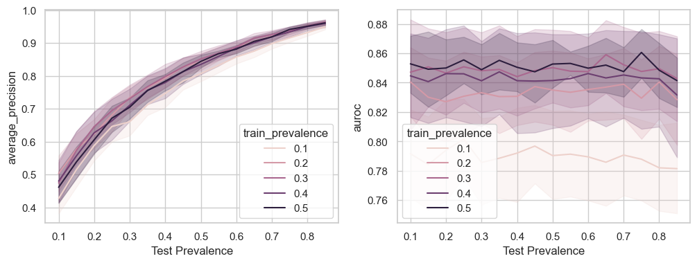
results = []

for p in [0.1, 0.2, 0.3, 0.4, 0.5]:
    # Run the simulation ten times for each prevalence to average out the noise
    for i in range(10):
        r = prevalence_sensitivity(n_samples, class_sep, n_clusters_per_class, (1-p, p))
        r['train_prevalence'] = p
        results.append(r)

results = pd.concat(results)

fig, axes = plt.subplots(1, 2, figsize=(12, 4))

for i, (m, ax) in enumerate(zip(['average_precision', 'auroc'], axes.flatten())):
    sns.lineplot(x='prevalence', y=m, hue='train_prevalence', data=results, ax=ax)
    ax.set_ylabel(m)
    ax.set_xlabel('Test Prevalence');

Based on this analysis, it appears that models trained across a variety of prevalence levels will have similar levels of precision for a fixed inference time prevalence, and all models will see an increase in precision as test time prevalence increases. The same cannot be said of AUROC which exhibits an almost “opposite” phenomenon: AUROC is invariant to test time prevalence, but varies greatly across models trained with different levels of training time prevalence.

So what’s the moral of this story? Nothing earth shattering, just a reemphasis of the fundamentals: get clear on what it is you are optimizing for and judiciously select metrics that allow you to isolate different aspects of performance related to that goal.